Lab 8: Conservation/Research Areas - Part 3 - Selecting Sites

This lab only contains instructions for ArcGIS Po. For ArcMap, please see the version of this lab for 2020.

Introduction

In the previous two labs, we found out where to acquire data, we performed a standardized quality control and quality assurance procedure, and we created data that we needed to complete the study. In this lab, we'll determine the best locations for studying and preserving the Coastal Giant Salamander (Dicamptodon tenebrosus). They like it wet so we need to find the best locations for them in Arcata Forest.

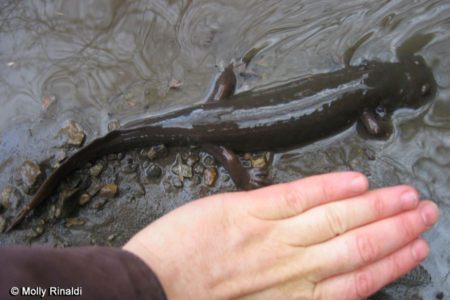
Image of a giant salamander and a hand

Photo courtesy of http://www.californiaherps.com.

Note: the instructor is not a biologist but thinks these salamanders are seriously cool. He created this lab based on what he could find out about the salamanders and then made up a few things to cover the GIS tools that you'll need in a wide variety of applications.

Learning Outcomes

After completing this lab, the student will be able to:

Use the field calculator
Use overlay operations: clip, buffer, dissolve, erase, etc.
Use "Select by Attribute"
Use the "Field Calculator"
Apply knowledge gained from previous lab exercises
Communicate the results of an analysis via a written report

Flow Chart

This lab has a lot of steps to it. You'll need to setup a new folder structure and then copy and project files either at the start of lab or as you need them. It is highly recommended that you create a new folder for this lab, make sure to keep everything you are working with in the same spatial reference, and go a good job naming data sets. I tend to add names to the end of a data set for each new step (i.e. Stream.shp, Stream_Buffer3m.shp, Stream_Buffer3m_Clip.shp). When I make a mistake I add a number to the end of the new data sets (i.e. Stream_Buffer1.shp, Stream_Buffer2.shp, etc.).

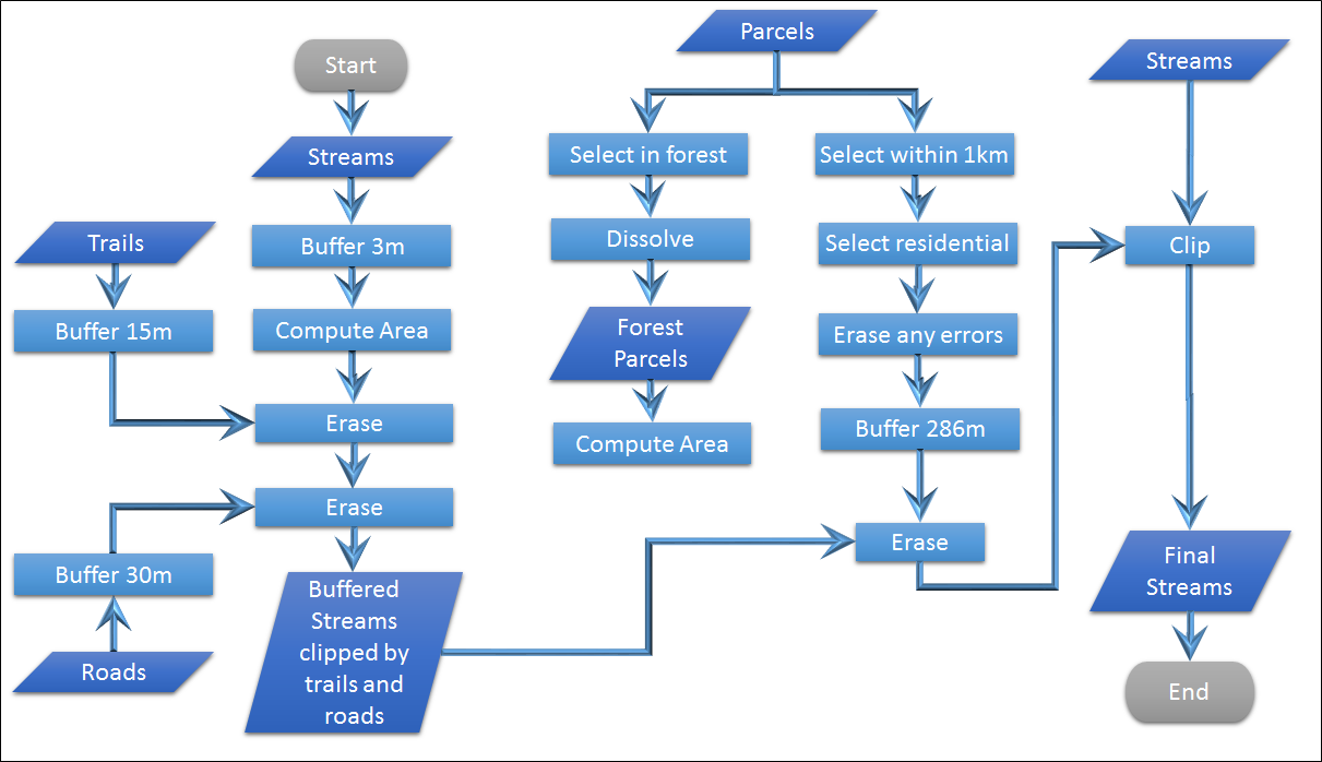
Creating the Stream Layer for Research

The flow chart below outlines the first half of the lab, creating a stream layer that includes the portions of the stream that are appropriate for research.

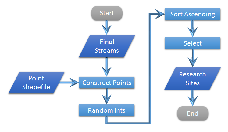
Selecting Sites

The second step is to select our final research sites.

Setting up Your Workspace

Setup you folder structure as in the past and include the data sets from the previous lab.

Create a folder structure and then copy the final streams, DEM, hillshade, and watersheds from the previous lab into the new workspace.
You'll also need the Arcata forest boundary, trails, and roads layers and the parcels shapefile for Humboldt County.
Make sure all these layers are in WGS 84 UTM Zone 10 North and place them in your working folder.

Note: For this lab, all work will be done using the spatial reference system:
WGS 84 UTM Zone 10 North

Habitat Near Streams

Defining the Habitat Near Streams

The next step is to define the habitat near streams. This would normally be much more complex to take into account the topography around a stream (i.e. the habitat would be narrower where the stream bank was steeper) but we'll simplify it here to just a horizontal buffer (which is used a lot for this type work, even when it probably should not).

Load the stream layer you created in the previous lab into ArcGIS Pro.
Open the "Buffer" tool .
Use your steam layer as the "Input Features".
Give the "Output Feature Class" a good name, like "Streams_Buffered_3m.shp".
Enter 3 meters for the "Linear Units" and select "OK".
Zoom in an note that your buffered streams are now polygons around your original streams layer. Buffering is another commonly used tool in GIS and can be used on points, polylines, and polygons.
Also notice that your streams have been "rounded" at the ends and now overlap the boundary of Arcata Forest. Go ahead and "Clip" them to the forest boundary now.
Then, zoom into where two of your stream reaches come together, see anything that might be a problem? The stream reaches were buffered individually and now overlap at the ends. If you compute the area using these polygons, the area will be larger than it should be. Use "Dissolve" to combine all the buffered stream areas into a single polygon.
Zoom in and checkout your stream buffers and see if they look correct.
As we did with "Length" for polylines in the last lab, add a "Field" to the "Attribute Table" and compute total the "Area" for these polygons. This will be the total area that we have for potential habitat.

Erasing Human Areas

Salamanders and humans (especially ones with dogs) do not mix well. Even though the city requires that dogs are always on a leash, visitors often violate that rule.

Buffer your roads to 30 meters (typical road easements are 15 meters plus another 15 for dogs to get off the trail) and buffer your trails to 15 meters
"Erase" the buffered road and trail shapes from the salamander habitat, enter the "Search" window and type "Erase". If you know the name of a tool in ArcGIS, this is the fastest way to find it. If you don't know the name, search the web for "ArcGIS <whatever you can come up with that might match the tool>" and you should find someone that has used the tool.
After the erase, zoom in an you should see the areas of the stream buffer have been erased around the roads and trails.

You should now have the habitat for salamanders that will avoid human trails and roads.

Note: If you open the attribute table, you'll see that your calculated area for the habitat has not changed! This will only update after you run the Calculate Geometry tool.

The Forest Boundary vs. the Parcels

Load the Arcata Forest boundary and the Humboldt County parcels layer.
Put the Arcata Forest boundary on top of the parcels layer and set it's fill to "no color".
How well do the boundaries between the two shapefiles line up? You might think this is unusual but it is not and it's often very difficult to find out what the "right" answer is.

For your report, note the maximum distance you can find between the lines in the two shapefiles.

We need to create a new boundary for Arcata Forest that matches the parcels shapefile as this might result in two different results.

First, we need to select the parcels and only those parcels that make up Arcata Forest in the county parcels layer. We also want to see the Arcata Forest boundary as we do this but it will be selected as well unless we turn off it's option for being selected. To do this, select the "List by Selection" icon in the table of contents.
Then, ArcGIS Pro: click on the checboxes to make other layers unselectable
Now, select the "Select Features" tool and click on one of the parcels that makes up Arcata Forest.
Hold down the "shift" key and select the other parcels until you have all of the parcels that make up Arcata Forest. Make sure you get them all as some of them are small.
If you're not sure which parcels are in the city, you can use the "info" tool to examine the parcels information and see which ones have a land use that indicates the parcel is in the Arcata Community Forest.
Then, return to the regular view in the Table of Contents and right click on the parcels layer and select "Data -> Export Data". Note that if there are selected features, they will be the only ones written out.
Give the new file a good name like "AracataForest_FromParcels.shp" and save it in your working folder.

Note: We do not recommend using "Create layer from selected features". This creates a temporary layer that stops working and crashes in a number of the tools. The process above is much more robust.

Note: This process of selecting data within a layer, creating a temporary layer, and then exporting it to a new shapefile is really common in GIS.

To make this into a single polygon, open the "Dissolve" tool .
Just select your new shapefile as the "Input Features", give the "Output Feature Class" a good name, and click "OK".
Take a look at the two boundaries and plan to include a map of their difference and the different computed areas in your report.
Make sure to clear any currently selected features.

Erasing the range of house cats in the parcels that border Arcata Forest

One of the issues with salamanders are predation by cats. Domestic cats will range a mean of 286 meters with a standard of deviation of 58 meters (Barratt, 1997). To remove this, we'll need to create a shapefile with the residential areas around the forest, buffer it, and then erase it from our habitat.

Finding the Cats!

Now we need to create a shapefile that just contains the parcels that might have house cats on them (we're going to ignore the feral cats).

Load the Polygon layer with the parcels.
Open the attribute table.
Open the "Select by Attribute" tool from the "Map" tab. This is a power tool for selecting features based on a verity of criteria. The easiest way to use the tool is to click on the buttons rather than typing.
In ArcGIS Pro:
1. For the WHERE clause,
2. Search in the "DESCRIPIO" field for text that "contains" something like "Residential"
3. Click "Run"
Take a look at the result against a background aerial image to see if any houses were missed. If so, add them by shift-clicking with the Select tool.
Create a new shapeile with your selection.

Removing the House Cat Home Range

We can now buffer our house cat home range to 286 meters to make sure our areas are at least beyond the mean range of house cats from their home.

Buffer the residential shapefile to 286 meters and erase it from the buffered stream layer.

You should now have a habitat map for salamanders that avoids humans, dogs, and cats. Remember to clip the habitat layer to the original Arcata Forest boundary and recompute the new area of habitat.

Final Stream Layer

As a final step, clip your original streams layer to the new habitat layer so we have streams to work with within the salamander habitat.

Note: You now probably have a large number of layers in ArcGIS Pro. This is a good time to remove most of them and just keep those we are going to use moving forward (i.e. the streams and buffered steams with areas erased that are poor habitat).

Selecting Research Sites

The next step is to define the sites where we will setup monitoring locations for salamanders. We want these to be along the streams and to be randomly placed. However, we also want to sample the full range of elevation that is available in the forest.

Load the stream layer you created above with all the buffered areas removed.
In ArcGIS Pro, Search for the "Generate Points Along Lines" tool.
Use the clipped steam layer for the "Input Features".
Give the output a good name.
Select "Distance" and enter "20" for the distance (i.e. 20 meters because we are in UTM).
Leave the other settings as they are and click "OK".
You should see points added to the point shapefile along the stream reach at a distance of 20 meters.

Random Attributes

We have far too many points for us to use for research but we want to have a statistically valid study of the area so we need to use a random approach to selecting the final sites.

Add a new attribute to the Research Sites data set with the name "Random" and the type of "Long" .
Right-click on the attribute header and select "Calculate Field". This will open another powerful tool in ArcGIS. This one allows you to compute new attribute/field values from other values.
Notice the "Random=" label over the panel in the bottom half of the dialog box. This is where you can type equations to compute the values in the attribute table. Type in "12" and then press "Run" . You should see all the values for "Random" be set to 12.
We're going to need to compute some random numbers which is not directly supported by the Field Calculator but can be computed using a little Python code which can be executed inside the Field Calculator (which is really cool!).
In ArcGIS Pro, select "Python 3" for the "Expression type"
Enter the code shown below in the "Code Block" panel. This is a Python function that will generate a random number that falls between a minimum and maximum value that you specify. The "import random" line imports the "random" function library into Python. The line with "return" calls the library to create a random number and then returns the value. Note that there are spaces in front of the second two lines. These let the parser know that these lines are part of the function and are very important.

def RandomInt(Min,Max):
 import random
 return random.randint(int(Min),int(Max))

Enter the code "RandomInt(0,100)" into the panel labeled "Random =". This code will call your function for each of the cells in the column that is selected (Make sure that you have the field labeled "Random" selected).
When done, you should see random (really pseudo random) values appear in the column.
Right-click on the column header and select "Sort Ascending".
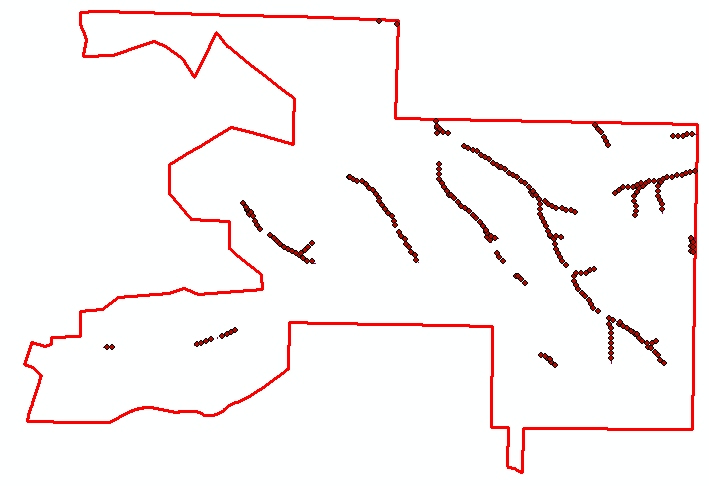
Select the first 10 rows in the attribute table. You should see 10 points along our steams highlight that are randomly placed.
Export these to a shapefile as your final research sites.

Stratified Random Sampling (Extra Credit/Optional and only partly updated for ArcGIS Pro!)

You may want to use stratified random sampling to say, make sure you include samples from different elevations.

The next step is to add the elevations from our DEM into the point file so we can select our sites. Load the filled DEM we created before.
Search for "Extract Points" and you'll see the tool "Extract Values to Points". Note that the search string does not have to match exactly, it just has to include a couple words in the name of the tool. Select the tool "Extract Values to Points".
Run the tool to create a new point shapefile.
Open the attribute table in the new shapefile and you should see a new column with the title "RASTERVALU". This column contains the values from our DEM that match the points!
The next step is to find the minimum and maximum elevation values. Right click on the "RASTERVALU" column heading and select "Statistics". This will show you the minimum and maximum values in the column. Record these values somewhere.
Create a new attribute called "Bins" as a "Short Integer".
Open "Calculate Field". Now double click on "RASTERVALU" in "Fields".
Notice that ArcGIS Pro puts exclamation points ("!") around RASTERVALU in the box below "Bins =". This indicates that the values in "Bins" should be replaced by the values from the "RASTERVALU" column. When you click "OK" you should see the values from "RASTERVALU" move into the "Bins" column but they will be converted to integer values because that is the type of the "Bins" attribute.
We want to make sure we have at least one bin in every 40 meters of elevation so we'll create a categorical attribute for each elevation band and then select sites within each band. Enter the following equation into Calculator Field replacing "Min" with the minimum RASTERVAL. Replace the Max-Min value with the maximum raster value minus the minimum value. This is the "range" of values within the raster. Replace the NumBins-1 with 4 (i.e. 5-1). The equation first subtracts the minimum value to move all elevations to 0 and then divides by the range of values. This converts the values to go from 0 to 1. Then, multiplies by the number of bins-1, 5 for this lab, to make the values go from 0 to 4 (notice that this is five bins). Recognize that the range of elevations for the bins will vary based on the range of values for your sites.
For ArcGIS Pro, put the equation below into the text field after "Bins=" but replace the brackets with explanation points "!".

( [RASTERVALU] - Min) / (Max-Min) * (NumBins-1)

In the next series of steps we are going to use "Select by Attribute" to select points that are in the same bin and then set the "Site" value to 1 for the two points with the lowest random values. We'll repeat this for each bin until we have our final sites.

Create a new attribute called "Site" with a long integer type .
Save your changes to the attribute table.
Use "Select by Attribute" to select the features that have a bin value of 0.
Make sure you have "Show selected records" selected at the bottom of the attribute table.
Right click on the "Random" field header and select "Sort Ascending".
Double click on the first row's "Site" value and change it to 1. Note that you can only edit these values after you save changes to the fields/attributes.
Change the second row's "Site" value to 1 as well. Now we have 2 sites selected in the first bin.
Repeat from step 3 for each of the bins.
After you've setup the "Site" attribute, select all the sites that have a value of 1 in "Site" and create a new shapefile from the selection.

Final Map

Create a final map of your study site and include labels for each of the study sites.

References

Barratt, D. G. 1997 Home range size, habitat utilization and movement patterns of suburban and farm cats Flis catus. Ecography, 20:271-280. <http://onlinelibrary.wiley.com/doi/10.1111/j.1600-0587.1997.tb00371.x/epdf>

Random Number Generator for the Field Calculator

Geospatial Activities